Bayesian A/B Testing at VWO

name: inverse
class: center, middle, inverse

# Bayesian A/B Testing at VWO
[Chris Stucchio](https://www.chrisstucchio.com) - [VWO](https://vwo.com)

---
## Multiple creative choices

![advertise on patch](patch_advertise_green.png)

---
## Multiple creative choices

![advertise on patch](patch_advertise_purple.png)

---
## Multiple creative choices

![advertise on patch](patch_advertise_pink.png)

---
class: center, middle
# Goal
## Find the one with the highest *conversion rate*

CR(version) = P( visitor buys advertising | version )

(In this example, purple.)

---
class: center, middle
# Motivation for Bayesian A/B testing

---
# A quiz

You've run an A/B test. Your A/B testing software has given you a p-value of $@ p = 0.03 $@ for a one-tailed test. Which of the following is true? (Note that several or none of the statements may be correct.)

1. You have disproved the null hypothesis (that is, there is no difference between the variations).
2. The probability of the null hypothesis being true is 0.03.
3. You have proved your experimental hypothesis (that the variation is better than the control).
4. The probability of the variation being better than control is 97%.
5. You know, if you decide to reject the null hypothesis, the probability that you are making the wrong
decision is 3%.
6. You have a reliable experimental finding in the sense that if the experiment were
repeated a great number of times, you would obtain a significant result on 97% of occasions.

---
class: center, middle
# All are false
## But try explaining that to customers...

[Misinterpretations of Significance: A Problem Students Share with Their Teachers?](http://myweb.brooklyn.liu.edu/cortiz/PDF%20Files/Misinterpretations%20of%20Significance.pdf)

(100% of psychology grad students and 80% of *Professors* got that quiz wrong.)

---
class: center, middle
# How does a Frequentist A/B test work?

---
## Formulate a null hypothesis.

The null hypothesis is the opposite of the thing you are trying to prove.

> In inferential statistics the null hypothesis usually refers to a general statement or default position that there is no relationship between two measured phenomena, or no difference among groups.[1] Rejecting or disproving the null hypothesis—and thus concluding that there are grounds for believing that there is a relationship between two phenomena (e.g. that a potential treatment has a measurable effect)—is a central task in the modern practice of science, and gives a precise sense in which a claim is capable of being proven false.

- [wikipedia](https://en.wikipedia.org/wiki/Null_hypothesis)

In web pages, this is usually the belief that the control group and the variation are equal.

---
## Gather data

- $@ i = \textrm{variation} $@. Control is $@ i = 0 $@, variation 1 is $@ i = 1 $@, etc.
- $@ c_i = \textrm{number of conversions} $@
- $@ n_i = \textrm{number of visitors} $@

Given this data, we can compute the *empirical* conversion rate:

$$
e_i = c_i / n_i
$$

---
## Derive test statistic

The *test statistic* is a number which should differ significantly from zero if the null hypothesis is false.

A good test statistic to take is the difference between the empirical conversion rates:

$$ \Delta e = e_1 - e_2 $$

---
## Assume null hypothesis is true

Assuming that the null hypothesis is true, find a probability distribution on the test statistic.

$$ q = (c_0+c_1)/(n_0+n_1) $$

$$ \Delta e \sim N\left(0, \sqrt{q(1-q)} \left(\frac{1}{n_0} + \frac{1}{n_1} \right)^{-1} \right)$$

(This last formula is only an approximation, based on the [central limit theorem](https://en.wikipedia.org/wiki/Central_limit_theorem). It's invalid for small $@ n_0 $@ and $@ n_1 $@.)

---
## Compute improbability of result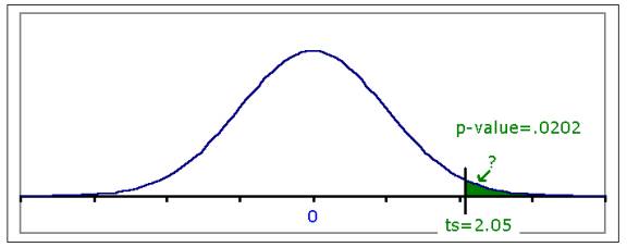

![p_value](p_value.jpg)

$$
p = P(x > \Delta e ~ | ~ \textrm{null hypothesis})
$$

The p-value is the probability of seeing a result at least as "extreme" as your real result if you ran an A/A test of the same size.

---
## Explaining the math doesn't make customers happy

![grumpy dog](grumpy_dog.jpg)

- Customers nearly always think it's the probability a mistake was made.
- Even our (VWO's) developers were (incorrectly) calling $@ 1 - p $@ the "chance to beat control". (We aren't unique - Optimizely called it the "chance to beat baseline.")

## Frequentist tests answer the wrong question!

---
class: center, middle
# Other confusion

---
## Repeated Peeks

>  the significance calculation makes a critical assumption that you have probably violated without even realizing it: that the sample size was fixed in advance. If instead of deciding ahead of time, “this experiment will collect exactly 1,000 observations,” you say, “we’ll run it until we see a significant difference,” all the reported significance levels become meaningless.

[Evan Miller, How Not to Run an A/B Test](http://www.evanmiller.org/how-not-to-run-an-ab-test.html)

(People do it anyway.)

---
## Repeated Peeks

![The peeking problem](peeking_problem.png)

P-value measures probability of crossing *green line*.

With repeated peeks, one is measuring the probability of crossing the *red line*.

---
# Uncertainty

>It had been six months since we started concerted A/B testing efforts at SumAll, and we had come to an uncomfortable conclusion: most of our winning results were not translating into improved user acquisition.

- [How Optimizely (Almost) Got Me Fired](http://blog.sumall.com/journal/optimizely-got-me-fired.html)

(Note: Optimizely is no more guilty than anyone else.)

Customers expect that if variation had 200 conversions out of 1000 visitors and control had 150/1000, they will get a 33% improvement. All such estimates come with quite a bit of uncertainty.

---
class: center, middle
# I'm a Bayesian
## because I'm not smart enough to be a Frequentist

![dumb dog](dumb_dog.jpg)

---
## Design goals for SmartStats

- Goal is to maximize revenue, not learn the truth.
- Customers want to know $@ P( \textrm{Variation B} > \textrm{Variation A} ) $@, not $@ P(x > \Delta e ~ | ~ \textrm{null hypothesis}) $@.
- Customers won't stop repeatedly peeking, so the statistics must allow this.
- Customers need to understand the uncertainty in the estimates.
- Customers are not experts, and will make mistakes if we allow it.

## Customer's real question: what do I do now to make the most money?
---
## Bayesian Philosophy

- There is a "real world", i.e. variation $@ i $@ has a conversion rate given by $@ \lambda_i $@. **We just don't know what it is.**
- Probability distribution $@ p(\lambda_i )$@ to represents our opinions about it.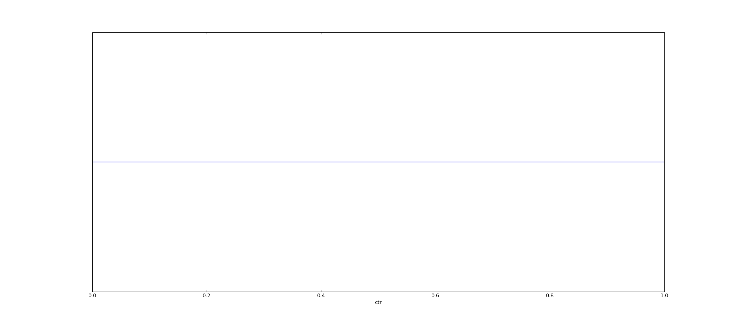

![test](example_pdf_1.png)
---
## Bayesian Philosophy

![test](example_pdf_2.png)

---
## Bayesian Philosophy

![test](example_pdf_3.png)

---
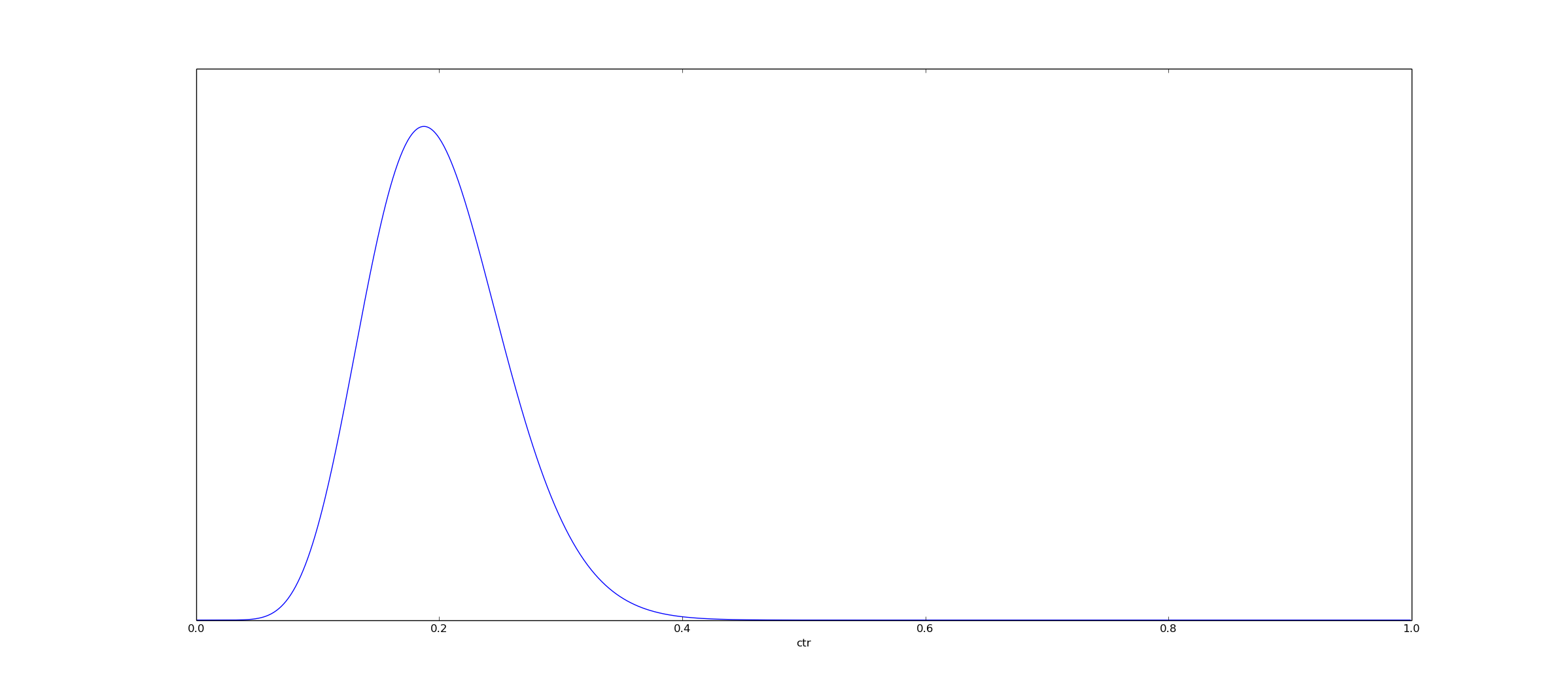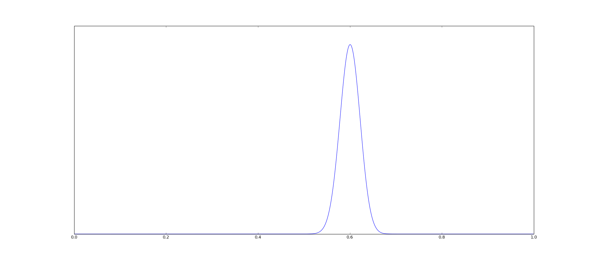## Bayesian Philosophy

Once we have a probability distribution, we can answer questions like "what is the probability the conversion rate is at least a and not more than b?"

$$
P(a \leq \lambda \leq b) = \int_a^b p(\lambda) d\lambda
$$

![test](event_illustration.png)

---
## Thinking in code

Consider a 100-element array p:

In [33]: p
    Out[33]:
    array([  1.81296534e-01,   1.49781508e-01,   1.23505113e-01,
             1.01637144e-01,   8.34724053e-02,   6.84129001e-02,
             ...
             4.98344117e-28,   2.10713975e-30,   9.50515970e-34,
             1.81296534e-39])

Suppose also:

In [29]: p.sum()
    Out[29]: 1.0000000000000004

and

In [29]: all(p >= 0)
    Out[29]: True

---
## Thinking in code

- `p[0]` represents the probability that the conversion rate is 0%
- `p[1]` represents the probability that the conversion rate is 1%
- etc

Then this:

$$
P(a \leq \lambda \leq b) = \int_a^b p(\lambda) d\lambda
$$

Is analogous to this:

p[int(100*a):int(100*b)].sum()

---
## Thinking in code

Another useful fact:

$$
E[f] = \int_a^b f(\lambda) p(\lambda) d\lambda
$$

Is analogous to this:

cr = [0.00, 0.01, 0.02, ..., 0.99]
    expected_value_of_f = ( p * f(cr) ).sum()

Here, `*` is standard pythonic element-wise multiplication.

(I call it `cr` rather than `lambda` because `lambda` is a keyword in python.)

---
class: center, middle
# "...when events change, I change my mind. What do you do?"
## Paul Samuelson

(Often incorrectly attributed to Keynes.)
---
class: center, middle
# Bayes Theorem
## The mathematically optimal way to change one's opinion

---
class: center, middle
$$
p\left(\lambda_i ~|~ \textrm{evidence}\right) = \frac{ p\left(\textrm{evidence} ~|~ \lambda_i \right) p(\lambda_i) }{ p(\textrm{evidence}) }
$$

---
# How to form an opinion
- Visitor arrived and converted.

$$
p\left(\lambda_i ~|~ \textrm{conversion}\right)
= \frac{ p\left(\textrm{conversion} ~|~ \lambda_i \right) p(\lambda_i) }{ p(\textrm{conversion}) }
= \frac{ \lambda_i p(\lambda_i) }{ p(\textrm{conversion}) }
$$

- Visitor arrived and did not convert:

$$
p\left(\lambda_i ~|~ \textrm{no conversion}\right)
= \frac{ p\left(\textrm{no conversion} ~|~ \lambda_i \right) p(\lambda_i) }{ p(\textrm{no conversion}) }
= \frac{ (1-\lambda_i) p(\lambda_i) }{ p(\textrm{no conversion}) }
$$

## Important math trick
Ignore the number on the bottom, $@ p(\textrm{no conversion}) $@ or $@ p(\textrm{conversion}) $@. This is a constant which doesn't change with $@ \lambda_i $@.

---
# How to form an opinion

What we believe before evidence.

$$ p(\lambda_i) $$

![prior](prior.png)

---
# How to form an opinion

What we believe after seeing one visitor who converts.

$$ \lambda_i p(\lambda_i) $$

![prior](posterior_one_click.png)

---
# How to form an opinion
This works recursively:

$$
p\left(\lambda_i ~|~ \textrm{2 conversions}\right)
= \frac{ p\left(\textrm{1 conversion} ~|~ \lambda_i \right) p(\lambda_i ~|~ \textrm{1 conversion} ) }{ p(\textrm{1 conversion}) }
$$
$$
= \frac{ p\left(\textrm{1 conversion} ~|~ \lambda_i \right) }{ p(\textrm{1 conversion}) }
\frac{ \lambda_i p(\lambda_i) }{ p(\textrm{1 conversion}) }
$$
$$
= \frac{ \lambda_i }{ p(\textrm{1 conversion}) }
\frac{ \lambda_i p(\lambda_i) }{ p(\textrm{1 conversion}) }
$$
$$
= C \lambda_i^2 p(\lambda_i)
$$

---
# How to form an opinion

$$
p\left(\lambda_i ~|~ c_i \textrm{ conversions}, n_i \textrm{visitors}\right) = C \lambda_i^{c_i} (1-\lambda_i)^{n_i - c_i} p(\lambda_i)
$$

## Mathematically optimal opinion about conversion rates

---
# How to form an opinion

What we believe before evidence.

$$ p(\lambda_i) $$

![prior](prior.png)

---
# How to form an opinion

What we believe after seeing one visitor who converts.

$$ \lambda_i p(\lambda_i) $$

![prior](posterior_one_click.png)

---
# How to form an opinion

What we believe after seeing one visitor who converts and 4 who do not.

$$ \lambda_i (1-\lambda_i)^4 p(\lambda_i) $$

![prior](posterior_one_click_4_noclick.png)

---
# How to form an opinion

What we believe after seeing one conversion, 21 non-converting visitors.

$$ \lambda_i (1-\lambda_i)^{21} p(\lambda_i) $$

![prior](posterior_one_click_20_noclick.png)

---
# How to form an opinion

What we believe after seeing 4 conversions, 203 non-converting visitors.

$$ \lambda_i^4 (1-\lambda_i)^{203} p(\lambda_i) $$

![prior](posterior_lots_of_displays.png)

---
# Joint Posterior
## Our opinion about the world

Want an opinion about all variations together, not each one individually.

$$
p(\lambda_0, \lambda_1, \ldots, \lambda_k) = p_0\left(\lambda_0 ~|~ \textrm{evidence} \right) p_1\left(\lambda_1 ~|~ \textrm{evidence} \right) \ldots p_k\left(\lambda_k ~|~ \textrm{evidence} \right)
$$

## Example

(For variation 0, 218 visitors and 12 conversions, for variation 2, 222 visitors and 19 conversions. Prior is taken to be 1.0.)

$$
p(\lambda_0, \lambda_1) = C \lambda_0^{12} (1-\lambda_0)^{206} 1.0 \cdot \lambda_1^{19} (1-\lambda_1)^{203} 1.0
$$

---

# Joint Posterior

![ab test posteriors](ab_test_posteriors.png)

---
# Joint Posterior

![ab test posteriors](ab_test_joint_probability_distribution.png)

---
# Decision rule

Want to minimize **regret** - the difference between the best choice and the choice we made. In a deterministic world:

$$
\textrm{regret}(i, \lambda_0, \ldots, \lambda_k) = \max_j \left( \lambda_j - \lambda_i \right)
$$

$$
= \max_{j \neq i} \left( \lambda_j - \lambda_i , 0\right)
$$

---
# Decision rule

But we don't actually know the true $@ (\lambda_0, \ldots, \lambda_k) $@ - all we have is an opinion about it.

So we compute the expected value based on our opinion:
$$
\textrm{regret}(i) = \int\ldots \int
\textrm{regret}(i, \lambda_0, \ldots, \lambda_k)
p(\lambda_0, \ldots, \lambda_k)
d\lambda_0 \ldots d\lambda_k
$$

---
# Decision rule

Choose regret tolerance $@ \epsilon $@ - a number small enough that you don't care about errors of this magnitude.

Run test until:

$$
\textrm{choice set} = \left[ i : \textrm{regret}(i) \leq \epsilon \right] \neq \emptyset
$$

At the end of the test, deploy as the smart decision any element from the choice set.

(Should be {} to denote set rather than [], but Mathjax.js isn't liking me today.)

---
# Uncertainty

Telling the user a single number for their conversion rate is a lie. The conversion rate could be many different values, so we emphasize the existence of a range:

![credible itnerval](reporting.jpg)

---
# Uncertainty

![creidlbe interval](credible_interval.png)

Ranges are called *credible* intervals. A 99% credible interval is region $@ [a,b] $@ for which:

$$
\int_a^b p_i(\lambda_i) d\lambda_i \geq 0.99
$$

---
# Lift is uncertain

"I made the call to action green and conversions went up 2%!" <- Another lie.

Users discover this a few weeks later when they deploy green and the 2% lift doesn't materialize.

A truthful statement:

![lift_display](display_lift.png)

---
# How to compute lift

Lift is $@ \lambda_1 - \lambda_0 $@, but how do we compute a probability distribution on this?

$$
u = \lambda_1 + \lambda_0
$$

$$
v = \lambda_1 - \lambda_0
$$

$$
p_{lift}(v) = \int p((1/2)(u-v), (1/2)(u+v))  du
$$

---
![lift graph](projection_graph.jpg)
---
# Easier to be exact

In many frequentist tests, applying the [Central Limit Theorem](https://en.wikipedia.org/wiki/Central_limit_theorem) is unavoidable. The Stats 101 formulae we previously used certainly did it.

The CLT works great when the number of samples is large.

![normal approx](normal_approximation.png)
---
# Easier to be exact

In many frequentist tests, applying the [Central Limit Theorem](https://en.wikipedia.org/wiki/Central_limit_theorem) is hard to avoid. The Stats 101 formulae we previously used certainly did it.

But not for small samples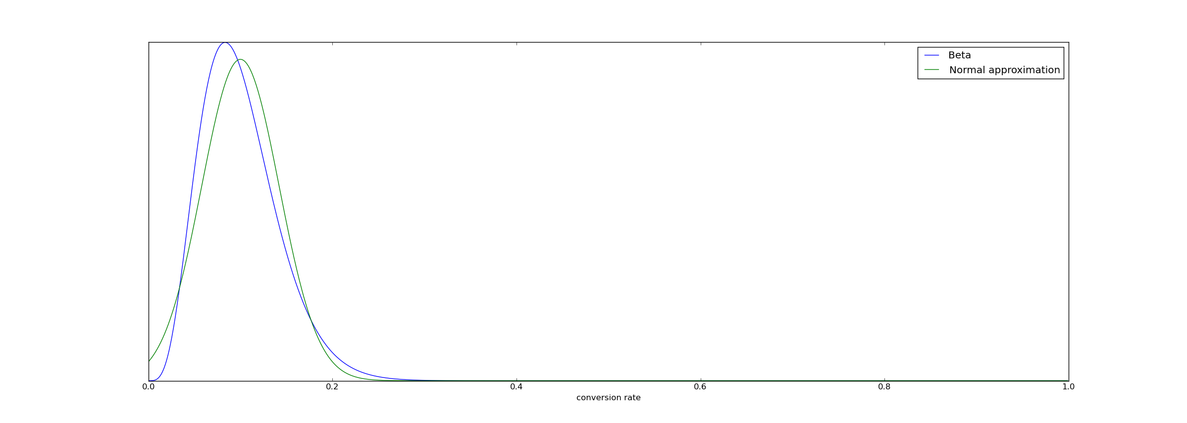

![normal approx](normal_approximation2.png)

---
# Easier to be exact

Part of the reason so many samples are required in frequentist tests is simply waiting for the CLT to work.

Bayesian statistics makes it more feasible to use exact arithmetic, and therefore use fewer samples.

---
# Revenue testing

Testing revenue is drastically faster, due to more careful math.

Fact: revenue for most visitors is zero. Distribution is "spike and slab" - big spike at zero revenue, everyone else widely distributed.

This is **very badly** approximated by a normal distribution.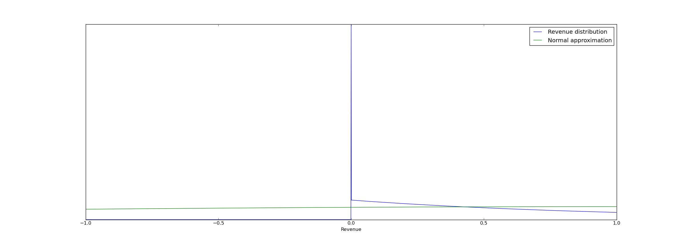

![normal approx](revenue_approximation.png)

---
# Revenue testing

For many revenue tests we can gain a 50-75% speedup over using CLT-based frequentist methods, due solely to this.

**Moral:** By modeling the true statistical process rather than an approximation, you avoid wasting samples learning things you already knew.

---
# Not *strictly* a Bayesian advantage

Using exact distributions rather than CLT is not inherently Bayesian. Many classical statisticians had the following methodology:

1. Solve the problem via a Bayesian method since it's easier to think about.
2. Realize that it's unpublishable.
3. Translate the Bayesian method back into Frequentist, get a p-value and publish.

During development of SmartStats I built a frequentist sequential test based on the spike+slab distribution. It was also a lot faster than CLT-based methods.

---
## So why does everyone do frequentist?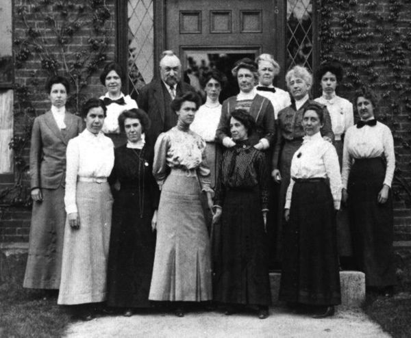

![old timey computer](pickering_computers.jpg)

Old school computers were slow.

---
## So why does everyone do frequentist?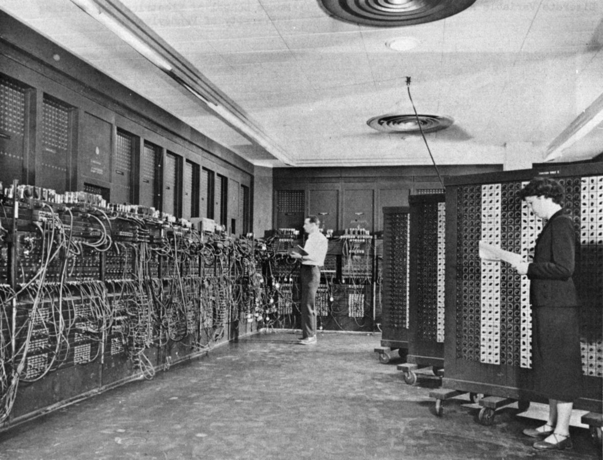

![old timey computer](old_timey.jpg)

---
## So why does everyone do frequentist?

- Frequentist calculations are 2-line Stats 101 formulas.
- Bayesian calculations have a 34 LaTeX document with lots of integrals.

- Frequentist calculations can be computed in microseconds in PHP.
- Bayesian calculations are minutes long monte carlo simulations - >95% of computing power at VWO is doing this.

## Monte Carlo is not fast

Me: "Why don't you offer better support for PDEs?"

Salesguy: "PDEs are a niche market. 20% of computing power in the world is devoted to monte carlo simulation."

---
# Conclusion

- Bayesian A/B testing helps us communicate our results more clearly to customers.
- Test concludes more rapidly because of revenue-optimizing tradeoffs, and better math.
- Better math is easier to do in the Bayesian framework.

- But it takes a lot more computing power.
---
# References

[VWO SmartStats Landing Page](https://vwo.com/bayesian-ab-testing/)

[Technical paper on VWO testing](http://cdn2.hubspot.net/hubfs/310840/VWO_SmartStats_technical_whitepaper.pdf) by me. Also a [more detailed tutorial](https://www.chrisstucchio.com/blog/2013/bayesian_analysis_conversion_rates.html) and [part 2](https://www.chrisstucchio.com/blog/2013/bayesian_bandit.html).

[Error Statistics](http://www.phil.vt.edu/dmayo/personal_website/Error_Statistics_2011.pdf), by Mayo and Spanos

[Statistical Methods Related to the Law of the Iterated Logarithm](http://projecteuclid.org/download/pdf_1/euclid.aoms/1177696786), by Robbins

[Further Optimal Regret Bounds for Thompson Sampling](http://jmlr.csail.mit.edu/proceedings/papers/v31/agrawal13a.pdf) by Agrawal and Goyal

[An investigation of the false discovery rate and misinterpretation of p-values](http://rsos.royalsocietypublishing.org/content/royopensci/1/3/140216.full.pdf), by Colquhoun

[Misinterpretations of Significance Problem Students Share with Their Teachers?](http://myweb.brooklyn.liu.edu/cortiz/PDF%20Files/Misinterpretations%20of%20Significance.pdf) by Haller & Krauss

[Robust misinterpretation of confidence intervals](http://www.ejwagenmakers.com/inpress/HoekstraEtAlPBR.pdf) by Hoekstra, Morey, Rouder & Wagenmakers